Aurora M. Ricart, Melissa Ward, Tessa M. Hill, Eric Sanford, Kristy J. Kroeker, Yuichiro Takeshita, Sarah Merolla, Priya Shukla, Aaron T. Ninokawa, Kristen Elsmore, Brian Gaylord
First published: 31 March 2021 https://doi.org/10.1111/gcb.15594
Abstract
Global‐scale ocean acidification has spurred interest in the capacity of seagrass ecosystems to increase seawater pH within crucial shoreline habitats through photosynthetic activity. However, the dynamic variability of the coastal carbonate system has impeded generalization into whether seagrass aerobic metabolism ameliorates low pH on physiologically and ecologically relevant timescales. Here we present results of the most extensive study to date of pH modulation by seagrasses, spanning seven meadows (Zostera marina) and 1000 km of U.S. west coast over 6 years. Amelioration by seagrass ecosystems compared to non‐vegetated areas occurred 65% of the time (mean increase 0.07 ± 0.008 SE). Events of continuous elevation in pH within seagrass ecosystems, indicating amelioration of low pH, were longer and of greater magnitude than opposing cases of reduced pH or exacerbation. Sustained elevations in pH of >0.1, comparable to a 30% decrease in [H+], were not restricted only to daylight hours but instead persisted for up to 21 days. Maximal pH elevations occurred in spring and summer during the seagrass growth season, with a tendency for stronger effects in higher latitude meadows. These results indicate that seagrass meadows can locally alleviate low pH conditions for extended periods of time with important implications for the conservation and management of coastal ecosystems.
1 INTRODUCTION
The oceanic uptake of anthropogenic carbon dioxide (CO2) is driving ocean acidification (OA) with a myriad of implications and threats for marine life (Kroeker et al., 2013; Orr et al., 2005). In particular, surface ocean pH has decreased globally by 0.1 pH units since the Industrial Revolution and is expected to decline an additional 0.3–0.4 pH units by the end of the century (Caldeira & Wickett, 2003). Furthermore, some geographic regions, such as those that experience coastal upwelling, are acidifying faster than others, highlighting the urgent need to explore mitigation strategies (Feely et al., 2008; Gruber et al., 2012; Osborne et al., 2020).
Photosynthesis in marine environments is a fundamental metabolic process that influences seawater pH, and the accompanying carbonate system more broadly, and can offset OA effects through uptake of CO2 and other forms of dissolved inorganic carbon (DIC) (Hendriks et al., 2014; Wahl et al., 2018). Elevation in pH occurs when photosynthesis dominates over respiration (Krause‐Jensen et al., 2016); this criterion applies to communities of habitat‐forming marine macrophytes (e.g., seagrasses and kelps) that inhabit coastal areas worldwide (Duarte & Cebrián, 1996). As a result, these ecosystems have been proposed as potential management tools to ameliorate low pH in coastal areas (Nielsen et al., 2018). Coastal areas, however, are typically characterized by large variability in environmental conditions driven by complex interactions among physical and biological processes (Waldbusser & Salisbury, 2014). These processes alter the coastal seawater carbonate system and induce appreciable fluctuations in pH. Such fluctuations eclipse the smaller variability of the open ocean and can dwarf the predicted decrease in average pH due to anthropogenic CO2 (Duarte et al., 2013; Hofmann et al., 2011; Kapsenberg & Cyronak, 2019). In particular, the metabolism of marine macrophytes often creates marked daily and seasonal fluctuations in pH (Camp et al., 2016; Hendriks et al., 2014; Krause‐Jensen et al., 2016; Manzello et al., 2012; Saderne et al., 2019; Silbiger & Sorte, 2018). As a consequence of this variability, the role of marine macrophytes in ameliorating exposure to low pH, in terms of timing, magnitude, extent, and relevance for organisms remains uncertain. For example, of the available studies in seagrass ecosystems, some suggest net amelioration of low pH (Buapet et al., 2013; Cyronak et al., 2018; Hendriks et al., 2014; Scanes et al., 2020; Su et al., 2020; Unsworth et al., 2012), while others suggest seagrasses may also amplify negative effects (Pacella et al., 2018). The limited spatial and temporal scales of prior studies further hinders understanding (Buapet et al., 2013; Cyronak et al., 2018; Hendriks et al., 2014; Pacella et al., 2018; Saderne et al., 2013, 2019; Semesi et al., 2009; Unsworth et al., 2012).
Here we present results of a study encompassing ~1000 km of coastline along the U.S. west coast that incorporates 6 years of data collected from seven seagrass meadows of Zostera marina, the most widespread seagrass species in the northern hemisphere (Green & Short, 2003). We deployed autonomous sensor packages in seagrass meadows to continuously record the seawater carbonate system for comparison to that of adjacent, non‐vegetated control areas. The sensors quantified in situ pH (total scale), dissolved oxygen, temperature, salinity, instantaneous water depth, and flow speed. We also collected data on seagrass morphological and ecosystem traits during each sensor deployment. We then defined “low pH amelioration” as the case when pH within a seagrass meadow exceeded that outside (i.e., positive ΔpH), and “low pH exacerbation” when ΔpH was negative. We explored relationships between ΔpH and potential biological, environmental, and hydrodynamic drivers to ascertain the primary controls on the seawater carbonate system in seagrass ecosystems. Our results demonstrate that, despite strong spatiotemporal variability, seagrass ecosystems can sustain prolonged periods of elevated seawater pH. This finding underscores that amelioration of low pH should join the list of other recognized ecosystem services provided by seagrasses, reinforcing the importance of protecting and restoring these habitats.
2 MATERIALS AND METHODS
2.1 Experimental design
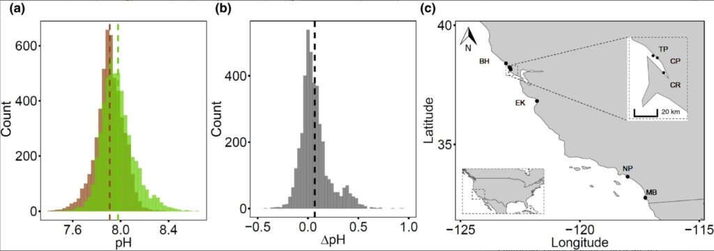
The study was performed at seven sites with Z. marina seagrass meadows spanning ~1000 km along the coast of California (Figure 1). The California coast includes two important oceanographic regions. Northern California, dominated by the California Current, is an upwelling region with cooler and more CO2‐rich waters brought up near the surface seasonally, while Southern California, dominated by the Southern California Countercurrent, is a region with less intense upwelling and where waters are warmer and less CO2 rich (Feely et al., 2016; Newman, 1979). The sites were selected along the different regions because of their similar estuarine geomorphological conditions (tidal estuaries), non‐carbonated muddy silicate sediments (less than ~7% of CaCO3), and the presence of Z. marina continuous seagrass meadows (larger than 0.5 km2) and non‐vegetated mud flats at similar depths (see Table S1 for more details).
The sensor packages were composed of a SeapHox (pH, temperature, salinity, dissolved oxygen, water pressure) or a SeaFET (pH, temperature) from SeaBird Scientific in combination with a MiniDot (dissolved oxygen, temperature) from Precision Measurement Engineering (PME). SeaFET and SeapHox pH sensors utilize the Honeywell Durafet combination electrode (Bresnahan et al., 2014; Martz et al., 2010; Takeshita et al., 2014). The sensor packages were attached to a metal frame and moored horizontally within the meadow’s canopy or unvegetated bottom on two metal poles anchored to the sediment with the sensing electrodes (SeaFET) and pump (SeapHox) situated 20 cm above the seafloor. Nortek Acoustic Doppler Velocimeters (ADV) were deployed within 1 m of each sensor package, one within the seagrass meadow and one outside in the non‐vegetated area. The ADV’s sensor heads were pointing upward to capture flow measurements at the canopy height, where data were collected every 2 h for a burst duration of 10 min, with a sampling frequency of 1 Hz. Some deployments happened simultaneously within the same site but at a different location within the seagrass meadow. As a consequence, not all deployments had corresponding ADV data.
Discrete water samples for pH and total alkalinity (AT) were collected over the duration of each deployment using a Niskin bottle immediately adjacent to the sensor during high tide. The water samples for pH were transferred to 250‐ml borosilicate glass bottles and preserved with 100 μl of saturated HgCl2 in cool temperatures (4°C), while the water samples for AT were transferred to 250‐ml plastic Nalgene bottles and frozen. Although alkalinity is largely conservative, freezing stops most of the biological activity assuring robust measurements without affecting results (data not shown). All samples were returned to the Bodega Marine Laboratory – University of California, Davis, for analysis. The number of discrete water samples varied from 2 to 10 per deployment, a subset of which included duplicates or triplicates. Additionally, salinity and temperature data were recorded at the same time of bottle sampling using a calibrated Yellow Springs Instruments Professional Plus Multiparameter meter (YSI ProPlus).
Honeywell Durafet pH sensors were calibrated based on field discrete water samples following best practices (Bresnahan et al., 2014). The pH was calculated from the internal reference electrode and reported in total scale at in situ temperature and salinity conditions (Rivest et al., 2016). The mean difference between reference samples and the sensor measurements was 0.01 (±0.006 SD), which meets the Global Ocean Acidification Observing Network (GOA‐ON) weather‐level data quality objectives and allows the use of pH data for the purposes of this study (Newton et al., 2014). Pressure data from SeapHOx sensors were calibrated with ADV pressure data from each deployment. Factory calibrations were used for the oxygen optodes (Aandera, SeapHOx; MiniDOts, PME) and salinity, and temperature (SBE‐37 MicroCAT, Seabird).
2.2 Sample analysis
Seawater pH of the discrete water samples was determined on the total scale with one of two high‐precision spectrophotometers using unpurified m‐cresol purple dye (Clayton & Byrne, 1993). A Submersible Autonomous Moored Instrument pH analyzer (SAMI‐pH; Lai et al., 2018; Martz et al., 2003; Seidel et al., 2008) from Sunburst modified for benchtop function was used from 2014 to 2017 (m‐cresol purple dye was prepared and calibrated by the manufacturer, sensors S80 07/23/12 and S83 06/12/14); and an Ocean Optics Jaz Spectrophotometer EL200 was used from 2017 to 2019 (m‐cresol purple dye from Sigma‐Aldrich, MKBR3556V and Acros Organics, AO394755 since 2019). Water samples were kept in a temperature‐controlled water bath (Thermo Scientific, Precision Microprocessor Controlled 280 Series) at 25°C before analysis to minimize temperature‐induced errors in absorbance measurements. Each pH instrument was validated by analyzing TRIS buffer revealing that the system was accurate to within 0.005 pH units. The carbonate system software package, CO2SYS Version 2.1 for MS Excel (Pierrot & Wallace, 2006), was used to calculate in situ pH values using in situ salinity and temperature measurements. Seawater AT was measured using open‐cell titration with triplicate samples (Metrohm 855 Robotic Titrosampler, Metrohm) using 0.1 N HCl (Fisher Chemical) diluted to a nominal concentration of 0.0125 M. Acid concentration was calibrated by analyzing Certified Reference Material (CRM) from A. Dickson’s laboratory before each titration session. For each set of triplicate analyses, the median value was considered. Instrumental precision from 50 of the analyses of CRM batches over the course of the study was SD <5 µmol kg−1. To provide a complete description of the seawater carbonate system (Table 1; Table S1), parameters were estimated from pH and AT, using the seacarb R package (Gattuso et al., 2019) and assuming published values for constants K1 and K2 (Lueker et al., 2000), Kf (Perez & Fraga, 1987), and Ks (Dickson, 1990). The AT in the time series was estimated from salinity values in sensors, based on linear regressions between salinity and AT of the discrete water samples. Independent regressions were done for each site (Bodega Harbor [BH]: R2 = 0.69, p < 0.001, df = 38; Tom’s Point [TP]: R2 = 0.33, p < 0.001, df = 32; Cypress Point [CP]: R2 = 0.76, p < 0.001, df = 22; Chicken Ranch [CR]: R2 = 0.52, p < 0.001, df = 9; Elkhorn Slough [EK]: R2 = 0.36, p < 0.001, df = 10; Newport Bay [NP]: R2 = 0.31, p < 0.001, df =15; Mission Bay [MB]: R2 = 0.25, p < 0.001, df = 26). Only pH values measured in situ are used for further data analysis. Uncertainties of the derived parameters (DIC, pCO2, and ΩAr) were quantified using a Monte Carlo analysis (100 simulations; Takeshita et al., 2021) on two deployments. These two deployments were chosen to represent a high (±38 μmol kg−1) and low (±8 μmol kg−1) uncertainty in the AT‐salinity relationship. For each simulation, normally distributed errors were introduced into pH (± 0.01) and AT (±25 μmol kg−1). The overall uncertainties of the derived parameters were calculated as one standard deviation of the simulations. On average, uncertainties for pCO2 (2.5%–3%) and ΩAr (0.02–0.05) were similar for both sites, as the calculations for these parameters are not particularly sensitive to AT. For pCO2, uncertainty is higher at lower pCO2, whereas uncertainty is lower for ΩAr at lower ΩAr. The uncertainty for DIC was similar to the uncertainty in AT, that is, ±33 and ±8.7 μmol kg−1 for the high and low AT uncertainty, respectively.
Note
- Estimated carbonate chemistry parameters were calculated for the whole dataset based on the relationship between salinity and total alkalinity from discrete samples (see methods, section 2.2).
- Abbreviations: ΩAr, aragonite saturation state; DIC, dissolved inorganic carbon; N, sample size of parameters measured in situ every 10 min, averaged per hour.
- a Total number of discrete samples.
2.3 Seagrass sampling
For each deployment, a 50 cm × 50 cm quadrat was deployed every 10 m in an 80 m linear transect starting at the sensor package within the seagrass meadow. In each quadrat, measures of shoot density were taken, and five seagrass shoots were collected and kept on ice during transport to the laboratory. In the laboratory, the longest leaf of each shoot was measured for maximum length and width. The seagrass leaf area index (LAI) was calculated as the average surface area of the leaf (length × width of the longest leaf) multiplied by the average seagrass shoot density (shoots m−2). LAI was chosen over other parameters because this metric integrates different structural parameters, reflecting the density of photosynthetic tissues, and has already been proposed as a main control of pH in seagrass meadows (Hendriks et al., 2014).
2.4 Statistical analysis
Data from sensors were excluded during times of sensor biofouling and/or sensor malfunctioning and obvious outliers (Bresnahan et al., 2014; Rivest et al., 2016). Prior to further analyses, two datasets were generated by averaging different time intervals, 1 h and 24 h. Then, each dataset was homogenized to achieve the same sample size per deployment. To homogenize sample size, a random selection of data was done on each sensor based on the data length of the shortest time series collected. Bootstrap iterative resampling (n = 1000) confirmed a negligible bias on the mean (<0.0001) and standard error (SE < 0.005) of each dataset for pH data in seagrass ecosystems and non‐vegetated areas. Then, we calculated the amelioration or exacerbation of low pH (ΔpH) in seagrass meadows by subtracting pH in the non‐vegetated areas from the pH in the seagrass ecosystems at each hourly or daily time point. Tables and figures show hourly averaged values unless otherwise indicated.
For each ADV record, mean velocity of the water flow (ū) was calculated as the vector sum of the two horizontal individual squared velocities, neglecting the much smaller vertical values, averaging across each burst and then further averaging per 24 h. Root mean square velocity (RMS water velocity) was calculated as the root mean square of the mean velocity of the water flow averaged per 24 h. This quantity serves as a measure of how much the individual velocity measurements fluctuate from the mean, and therefore provides a simple metric of overall water motion, which among other effects, acts to disperse and dilute the metabolic signature of the seagrass in seawater chemistry.
We used linear simple models (LM) to evaluate the relationship between pH and dissolved oxygen in seagrass meadows and non‐vegetated areas, and also to check for differences in the duration of events of low pH amelioration above a certain ΔpH threshold. In both cases we used the complete time series. For the latter, we took the most conservative approach to calculate the duration of events, as we considered events to be distinct even when ΔpH decreased below the chosen threshold for just 10 min. We used linear mixed effects models (LMMs) to determine how pH varied as a function of the type of habitat (seagrass vs. non‐vegetated), and how ΔpH varied as a function of day–night light periods, season of the year, seagrass productivity period, and sites. Day–night light periods were classified based on sunrise and sunset times per each day. Seasons of the year were classified based on the four divisions of the year in temperate areas. Seagrass productivity periods were classified based on the growth season (April through September) and senescence season (October through March) for the seagrass species Z. marina in California. All these models were run with the independent categorical variable of interest as the fixed effect and deployment as the random effect (fixed slope, varying intercept). To avoid biases based on the unbalanced design, for the comparison between seasons we only included the sites that presented data in most seasons; and we only included data from spring and summer for the comparison among sites, as data from these seasons were available for all sites. All the LMMs were developed with the dataset averaged by 24 h time intervals except for the day–night light period comparison where we used the dataset averaged by 1 h time intervals. Models were generated with the lme4 R package (Bates et al., 2014). Before full models were generated, the applied random effect was determined by contrasting null models with different random structures: deployment, deployment within each site, and deployment within each season. Best random structure (i.e., deployment) was chosen by performing a likelihood ratio chi‐square test to assess model significance, which tests whether reduction in the residual sum of squares is statistically significant or not. The significance of the fixed effects was evaluated by comparing each full model to the null model performing a likelihood ratio chi‐square test, and also comparing Akaike’s information criterion (AIC). Fixed effects were considered for AIC differences bigger than 2 and a p < 0.05. Normality and homoscedasticity were explored via visual estimation of trends of model residuals (errors associated with homogeneity of variance, independence, and normality). Temporal autocorrelation on model residuals was assessed by plotting autocorrelation function coefficients as a function of lag k (abscissa) in correlograms.
We used principal component analysis (PCA) to assess the relationships between environmental and biological controls and the seagrass amelioration of low pH. In particular, we examined the relationships among seagrass amelioration or exacerbation of low pH (ΔpH), daylength, pH in seagrass, temperature, pCO2 of the surrounding water (that from non‐vegetated areas), water column height, RMS water velocity, and seagrass LAI. The PCA was developed with the dataset averaged by 24 h time intervals. All data were standardized to account for differences in measurement units. For standardization, we subtracted the minimum from the value of interest, and then divided by the difference between the maximum and minimum value.
3 RESULTS
3.1 The seagrass seawater carbonate system and the amelioration of low pH
Seagrass ecosystems in our study exhibited higher average pH in comparison to non‐vegetated areas (null vs. full LMM, χ2 = 81.227, df = 1, p < 0.001, Table S1), with a mean pH of 7.98 ± 0.002 SE within seagrass ecosystems, and a mean pH of 7.91 ± 0.001 SE in non‐vegetated areas (Figure 1a; Table 1). Extreme values of pH also differed across these environments. Maximal values of pH were achieved within seagrass ecosystems (pH = 8.60), while pH minima were similar between seagrass ecosystems and non‐vegetated areas (pH ~ 7.4; Figure 1a; Table 1). Overall, the pH was higher in seagrass ecosystems for 65% of the measurements (Figure 1b).
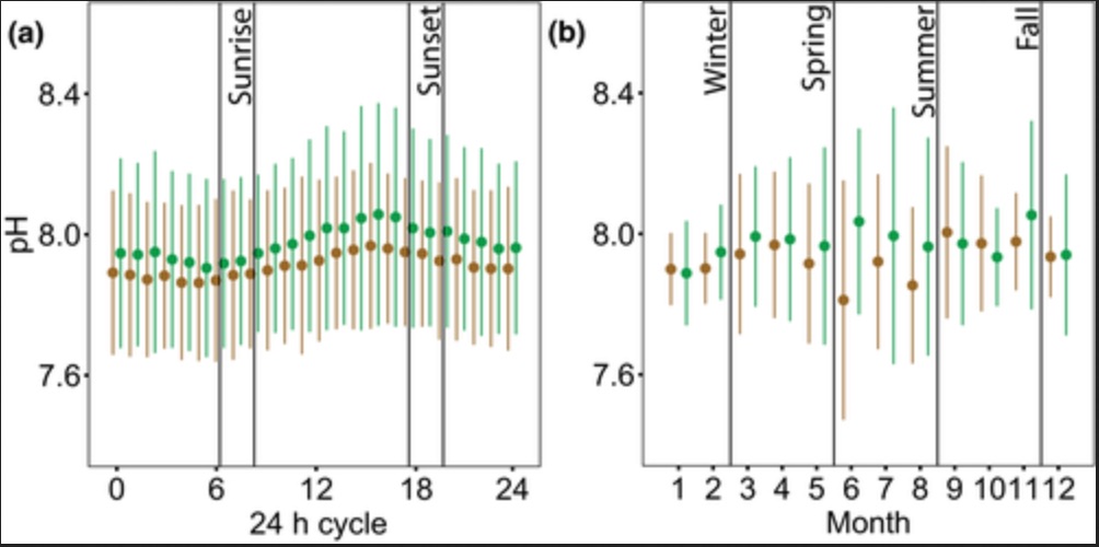
All pH time series collected in this study exhibited high‐frequency daily fluctuations (Figure S1). The amplitude of pH daily fluctuations, or maximum change of pH over a 24‐h cycle, was as high as 0.97 pH units, with an average amplitude of 0.29 ± 0.007 SE, for seagrass and up to 0.92 pH units, with an average amplitude of 0.23 ± 0.005 SE, for non‐vegetated areas. Four dominant patterns capture the characteristics of when and how low pH amelioration or exacerbation arises (Figure 2; Figure S1). From the most common pattern to the least common, we observed: (1) a positive offset where pH is uniformly higher in seagrass ecosystems (Figure 2a); (2) similar pH minima in both seagrass and non‐vegetated areas with excursions to relatively higher pH values during the day in seagrass ecosystems (Figure 2b); (3) a negative offset (Figure 2c); (4) similar baseline with a higher pH in seagrass during the day but lower pH during the night compared with non‐vegetated areas that have less variability (Figure 2d). The relationship between pH and dissolved oxygen concentration illustrates the coupling between primary productivity and carbonate chemistry, and thus indicates that the metabolic activities of photosynthesis and respiration largely control pH in seagrass ecosystems and in non‐vegetated areas (linear regression, for seagrass: R2 = 0.43, df = 96,091, p < 0.001; for non‐vegetated areas: R2 = 0.39, df = 79,286, p < 0.001), although other processes likely also contribute to variation in pH. These different patterns (Figure 2) were sometimes present during the same deployment (Figure S1), suggesting that drivers such as hydrodynamic or environmental factors may modulate the metabolic pH signal (Cyronak et al., 2018, 2020; Hendriks et al., 2014; Hurd, 2015; James et al., 2020; Koweek et al., 2018). In addition, trends in the pH time series (i.e., an increase or decrease in mean pH over several days), if found, were coincident in seagrass and non‐vegetated areas, and were related to tidal cycles (Figure S1).
![]()
3.2 Temporal and spatial variability of the amelioration of low pH in seagrass ecosystems
Amelioration of low pH occurred in both daytime and nighttime, where the differences in ΔpH between daytime and nighttime were trivial but marginally higher at night (null vs. full LMM, χ2 = 15.997, df = 1, p < 0.001; Figure 5a; Table S2). This finding confirms that, in most cases, the increase in pH inside seagrass beds relative to the non‐vegetated areas observed during the day is maintained throughout the night (e.g., Figure 2a), such that even during the nighttime, seagrass meadows can still be influenced by preceding daytime buffering. Differences in ΔpH were significant among seasons (null vs. full LMMfour seasons, χ2 = 14.405, df = 3, p = 0.002; null vs. full LMMgrowth vs. senescence, χ2 = 14.34, df = 1, p < 0.001). The extent of low pH amelioration was higher in spring and summer and declined in fall and winter (Figure 5b; Table S2), with higher amelioration coincident with the active growth season of the plants (Figure 5c; Table S2). Differences in ΔpH were also apparent among sites (null vs. full LMM, χ2 = 14.798, df = 6, p = 0.022), with a trend toward amelioration in northern sites and no amelioration or even exacerbation in southern sites (Figure 5d; Table S2).
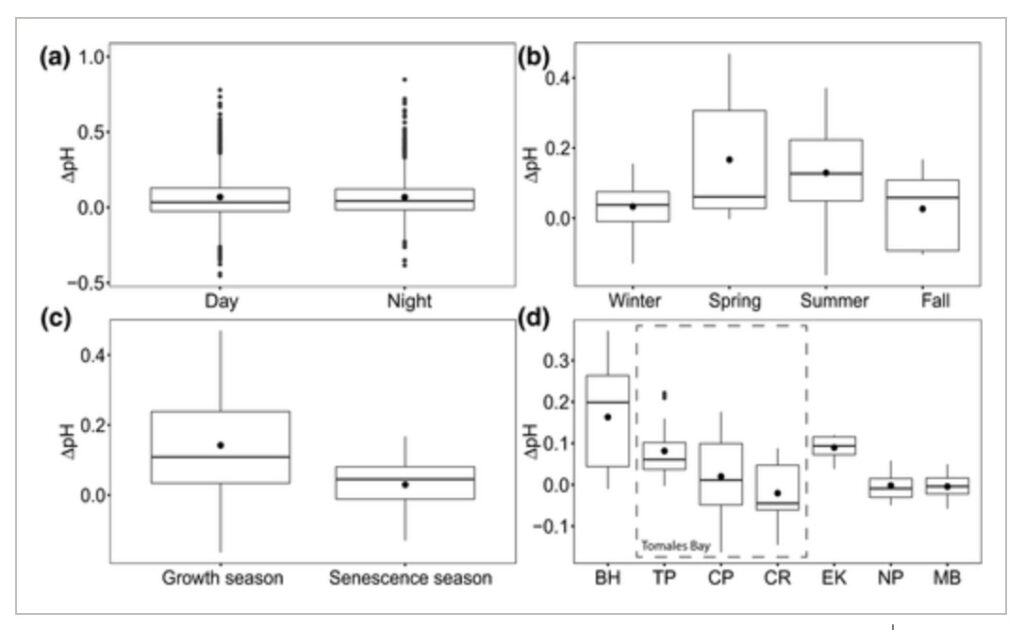
Figure 5
Temporal and spatial variability of the amelioration or exacerbation of low pH in seagrass ecosystems. (a) ΔpH during daytime compared to ΔpH during nighttime (nday =2267 h, nnight =2083 h, n = 150 h/deployment; n = 29 deployments); (b) comparison of ΔpH among seasons, only including sites sampled in most seasons (BH, TP, CP), (nwinter =34 days, nspring =32 days, nsummer =64 days, nfall =22 days; n = 8 days/deployment; n = 19 deployments); (c) comparison of ΔpH between seagrass productivity periods, only including sites sampled in most seasons (BH, TP, CP), (ngrowth =96 days, nsenescence =56 days; n = 8 days/deployment; n = 19 deployments); (d) comparison of ΔpH among sites, only including spring and summer seasons (nBH =48 days, nTP =24 days, nCP =24 days, nCR =8 days, nEK =8 days, nNP =24 days, nMB =16 days; n = 8 days/deployment; n = 19 deployments). Sites in panel (d) are ordered from north to south, from left to right, including three seagrass meadows within Tomales Bay. See Figure 1 for full site names. Data points in (a) represent hourly averages from each deployment. Data points in (b), (c), and (d) represent daily averages from each deployment. Boxplots represent median and quartiles (0.25, 0.75), whiskers represent scores inside the 1.5*Interquartile range (IQR). Mean values are shown with a black dot within the box
3.3 Controls on seagrass amelioration of low pH
The synchronicity of biological and environmental factors that increase seawater pH (e.g., photosynthesis, temperature, irradiance) with favorable seawater hydrodynamics (e.g., slack low tides with limited water movement) likely drive patterns of amelioration of low pH (ΔpH) in seagrass ecosystems (Koweek et al., 2018). Using a PCA, we assessed the relationships between ΔpH and multiple potential drivers (Figure 6). A PCA is often used to reduce the dimensionality of large datasets, by transforming a large set of variables that are usually correlated into a set of orthogonal “principal components” that specify the main axes of total variation across all parameters. The first and second principal components are of special interest because they explain the highest proportion of the total variance. Here, the first principal component explained 35.7% of the total variance and captured strong seasonal differences (see points that are from summer on the right, and winter and fall on the left of Figure 6). We also see the ΔpH vector aligned closely with the first principal component, indicating a positive correlation (r = 0.49). Likewise, positive correlations were found between the first principal component and temperature (r = 0.38), daylength (r = 0.48), LAI (r = 0.34), and pH within seagrass (r = 0.40). All of these factors would be expected to positively influence the capacity of seagrass meadows to uptake DIC through photosynthesis (Fourqurean et al., 1997; García‐Reyes & Largier, 2012; Hendriks et al., 2014). In contrast, negative correlations were apparent between the first principal component and water height (r = −0.22) and the RMS of water velocity (r = −0.14). RMS velocity provides a rough metric of overall water motion within a seagrass meadow, and thus, the strength of dispersion processes that reduce water residence time. The factors of water height and RMS velocity therefore characterize together two fluid dynamic properties that tend to decrease the seagrass capacity to alter seawater chemistry by diluting and dispersing the signature of plant metabolic processes. Thus, greater water depth and water flushing rates would be expected to decrease the magnitude of ΔpH. The second principal component explained 18.8% of the total variance and was negatively correlated with the pCO2 of the surrounding water (r = −0.64), temperature (r = −0.24), water height (r = −0.43) and positively correlated with pH within seagrass (r = 0.47). Many of these latter factors can vary geographically and over shorter time periods than season, and the second principal component may capture aspects of this higher frequency variability, especially during the summer season (see high dispersion of blue points).
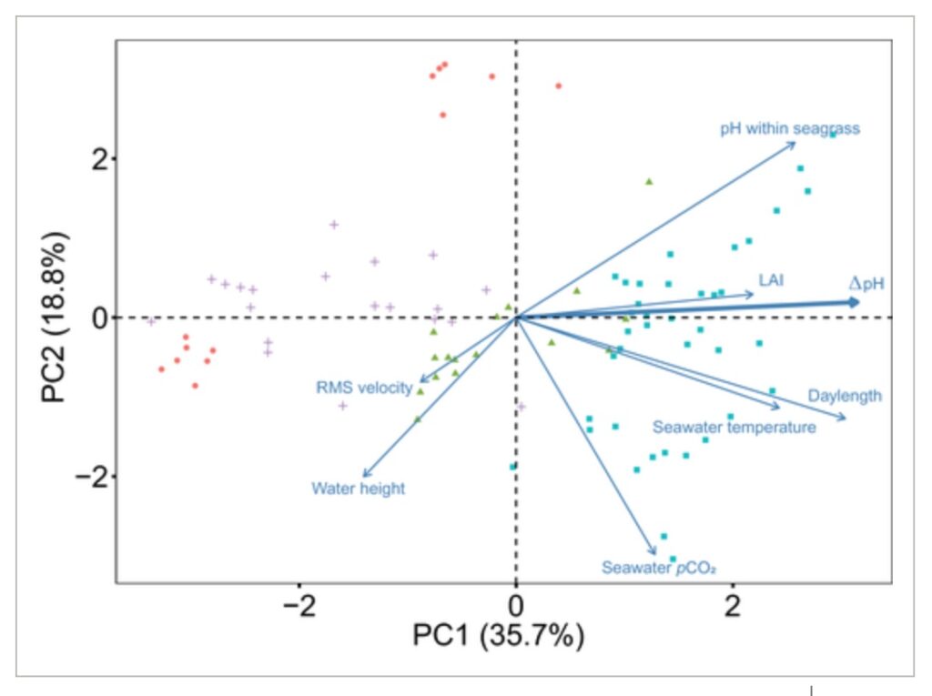
Figure 6
Principal component analysis of the controls of the amelioration of low pH in seagrass ecosystems. Biplot of variable vectors showing the correlation between the variables, the principal components, and individual factors. The direction of the arrows is determined by the eigenvectors that relate each variable to the two primary principal components. The direction of the arrows indicates that the values of that variable increase in that direction. Data points represent daily averages from each deployment. Colors represent the different seasons measured: blue squares = summer; green triangles = spring; red circles = fall; purple crosses = winter. Abbreviations for the individual factors are as follows: LAI = leaf area index; RMS velocity = root mean square water velocity; seawater pCO2 = partial pressure of CO2 in the non‐vegetated areas
4 DISCUSSION
4.1 Potential for seagrass ecosystems to ameliorate low pH in coastal areas and management implications
Our study is the most extensive in situ high‐frequency assessment of pH in seagrass meadows to date. It confirms, through empirical evidence collected across broad oceanographic and biogeographic regions (Feely et al., 2016; Newman, 1979), that pH tends to be higher within seagrass ecosystems compared with adjacent non‐vegetated areas. Important seasonal and geographic patterns modulate this broad trend, where the magnitude and duration of pH amelioration events within seagrass meadows are larger than those of pH exacerbation events. Consistent with prior studies (Frankignoulle & Distèche, 1984; Hendriks et al., 2014), the highest amelioration of low pH is observed during spring and summer, coincident with the peak of productivity and growth of temperate seagrasses. This finding, together with the coupling found between pH and DO, indicates that aerobic metabolism dominates the reported patterns. However, other processes might be involved, as the correlation between pH and DO presented some anomalies (i.e., low R2). The shorter air–sea exchange timescale for oxygen compared to CO2, or a decoupling between decomposition and primary production driven by mixing of water masses, might also contribute to these results but requires further exploration (Lowe et al., 2019).
Our results also suggest the existence of geographic variation in the amelioration of low pH by seagrass ecosystems that may be related to different, potentially interactive processes. During spring and early summer, upwelling events are characteristic at our northern study sites (Feely et al., 2008; García‐Reyes & Largier, 2012) and may increase seagrass photosynthetic rates due to the oceanographic influx of nutrients and aqueous CO2 into the coastal zone (Invers et al., 2001; Koch et al., 2013; Zimmerman et al., 2017). The highest amelioration of low pH is found in the northern sites that are more exposed to the open ocean (see the gradient within Tomales Bay, Figure 5) and tend to experience stronger, more sustained upwelling events compared to southern sites. In addition, there is strong morphological variation in seagrass species traits between northern and southern sites (e.g., we found longer seagrass leaves in the north) that are likely to drive higher seagrass productivity and greater amelioration of low pH in the northern sites, although photosynthetic rates were not measured in our study. Seagrass physiology and the effects of biotic and abiotic environmental drivers on seagrass metabolism are well studied, but our understanding of how those factors, in combination, affect the seawater carbonate system is still limited, since many of the drivers discussed above can also affect the seawater carbonate system independent of the seagrass metabolism. Such complexity highlights the need for further studies to fully discern the importance of different controls of pH in seagrass ecosystems and direct the selection of sites where the amelioration of low pH by seagrasses could be an effective OA management strategy.
Although our study characterizes the effect of seagrass on the seawater carbonate system, it remains unclear how these chemical changes might influence the responses of calcifying and non‐calcifying organisms associated with these ecosystems. Many species that live within or very close to seagrass meadows are considered highly vulnerable to OA (Barton et al., 2012; Groner et al., 2018; Hettinger et al., 2013; Miller et al., 2016; Thomsen et al., 2015). Some examples in the study area are the oysters Ostrea lurida and Crassostrea gigas (the latter being a non‐native species mostly found in on‐site aquaculture facilities) and the Dungeness crab Cancer magister (which is the basis of an economically important fishery along the U.S. west coast). Impacts to physiological or ecological performance in these species can occur with more modest pH reductions than the elevations in pH that we observed in seagrass meadows (Barton et al., 2012; Groner et al., 2018; Miller et al., 2016; Thomsen et al., 2015). However, sensitivity to OA is driven not only by the intensity of exposure but also its duration (Waldbusser et al., 2015; Waldbusser & Salisbury, 2014). Yet, for most organisms we do not know if thresholds in the intensity or duration of low pH events exist that would critically impact performance, as most of the research has only used two or three static mean pH values for exposure (Kroeker et al., 2010, 2013). Thus, it is still unknown whether organisms are most sensitive to changes in mean versus minimum or maximum pH, and how these sensitivities might vary among response variables (e.g., calcification, growth, survival). Moreover, other environmental stressors (e.g., temperature, turbidity) can preclude organisms to benefit from the favorable carbonate chemistry. There are also many complex community interactions that must be considered when exploring the ability of seagrasses to ameliorate OA to a degree that will have a net positive benefit to particular species (e.g., predation risk can be higher within a seagrass meadow; Lowe et al., 2019). Additional paired chemical and biological studies should focus on addressing these gaps.
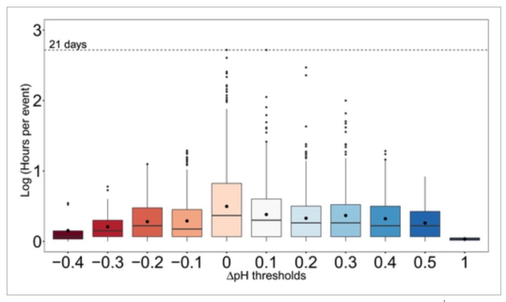
Although longer term amelioration of low pH may have greater potential benefits in general, short‐term carbon drawdown on hourly to daily scales can be especially important when such events coincide with times of heightened organismal sensitivity such as during a species’ early life stages (i.e., larvae; Waldbusser et al., 2013). OA refugia are most relevant to sensitive organisms particularly when exposed to undersaturated waters (Kroeker et al., 2013; Waldbusser & Salisbury, 2014). In upwelling areas, those conditions often occur in spring and summer, aligning with times when seagrass pH amelioration was also highest. Our results suggest that seagrass ecosystems could protect vulnerable organisms from extreme episodic pH conditions and provide temporary chemical refugia to improve calcification and/or limit the time spent below critical physiological thresholds in pH. Moreover, this study demonstrates how amelioration of low pH can extend over physiologically and ecologically relevant timescales (e.g., elevations of pH higher than 0.1 for up 21 days, or higher than 0.3 for up to 4 days), and counters concerns that marine macrophytes might only confer OA refugia during daytime hours (Hendriks et al., 2014; Kapsenberg & Cyronak, 2019; Middelboe & Hansen, 2007; Semesi et al., 2009).
Enhanced carbon sequestration through conservation and restoration of vegetated ecosystems is of crucial importance for future scenarios of climate change (IPCC, 2014). Seagrass ecosystems are recognized as important carbon sinks that can reduce global atmospheric CO2 concentrations through burial of organic carbon and long‐term storage within the sediments (Fourqurean et al., 2012; Kennedy et al., 2010). As a result, seagrasses are now being considered in national greenhouse gas reduction schemes (Hiraishi et al., 2013; Serrano et al., 2019; Thomas, 2014). We present evidence supporting that in addition to their global role in carbon sequestration, seagrass ecosystems could also be leveraged as local management tools to mitigate the consequences of OA. Moreover, seagrasses are understood to be currently limited by CO2 availability (Koch et al., 2013) and an increase in CO2 concentration in the water due to OA is expected to increase their productivity (Sand‐Jensen et al., 2007; Zimmerman et al., 2015, 2017) which in turn could enhance their capacity to increase pH even as pH decreases over the next years. Our work strongly indicates the potential for seagrasses to mitigate low pH in coastal areas and has important implications for the conservation and management of seagrass ecosystems.
ACKNOWLEDGMENTS
This study was supported by the California Sea Grant (Award R/HCME‐03 to Hill, Gaylord, Sanford) and the California Ocean Protection Council. We thank Grant Susner, Katie Nichols, Gabriel Ng, Scott Gabara, Josep Miàs, Sarah Lummis, Jason Toy, Evan O’Brien, Brent Hughes, Luis Hernández, and Shannon Meyers for their help in the field and/or the laboratory. We also thank Kevin Hovel and Jay Stachowicz for their help with scientific collecting permits. This work was performed in part at the University of California Natural Reserve System Kendall‐Frost Mission Bay Marsh Reserve, https://doi.org/10.21973/N3008B.
CONFLICT OF INTEREST
The authors declare no conflicting interests.
AUTHOR CONTRIBUTIONS
Aurora M. Ricart, Melissa Ward, Tessa M. Hill, Eric Sanford, Kristy J. Kroeker, Yuichiro Takeshita, and Brian Gaylord conceived and designed methodology. Aurora M. Ricart, Melissa Ward, Kristy J. Kroeker, Yuichiro Takeshita, Sarah Merolla, Priya Shukla, and Aaron T. Ninokawa collected the data. Aurora M. Ricart, Brian Gaylord, Yuichiro Takeshita, Kristen Elsmore, and Aaron T. Ninokawa analyzed the data. Aurora M. Ricart led the writing of the manuscript. All authors contributed critically to the drafts and gave final approval for publication.
Original post: https://onlinelibrary.wiley.com/doi/10.1111/gcb.15594